Machine Learning: A gentle introduction
machine-learning
ai
Looking at the last Google and Apple conventions it was clear to all: if in the past years the main buzzwords in the information technology field were IoT and Big Data, the catch’em all word of this year is without any doubts Machine Learning. What does this word exactly means? Are we talking about artificial intelligence? Somebody is trying to build a Skynet to ruin the world? Machines will steal my job in the future? “Know your enemy”, they said. So let’s try to understand what Machine Learning really means.
Definitions
The task we are going to accomplish is not simple. So, let’s start from the beginning: What does machine learning refer to.
Machine Learning is a discipline of Artificial Intelligence, that is responsible to study and develop algorithms that allows machines to learn information. In detail, the learning process is done using an inductive approach, that tries to extract rules and behavioural patterns from huge amount of data.
The types of information used by the algorithms (learners) to learn identify the following categorization of machine learning algorithms, which are:
- Supervised learning: The learner exploits a set of given couples (input, output) to learn a function \(f\) that maps input to output. The above couples are called supervisions and using them the learner tries to find the function that approximately fits like \(f\). Supervisions must be available at the beginning of the learning process.
- Unsupervised learning: In this kind of learning process, the function \(f\) is learned by the learner using solely the given inputs. There is no a priori information relative to the output of the function \(f\). In this type of learning process, the learner tries to approximate the probability distribution of the given inputs.
- Reinforcement learning: Given an environment which an agent can interact with and given a set of positive and negative returns the environment can give to the agent, the objective in this case is to find a policy of action of the agent that maximizes the values of the above returns.
Let we look at some examples. We have some food, i.e. pasta, oranges, apples and chocolate. Using a supervised approach we give to the learner the whole set of foods, specifying which of these is a fruit and which is not. Using this information, the learner tries to understand what features fruits have. Given a new food , the algorithm will try to guess if it is a fruit or not.
Using an unsupervised approach, we do not know the type of each food. Our task is to group each piece with something that seems to be similar. The learner will try to build these groups (or clusters) looking at the information it has.
In reinforcement learning, the food is all scattered on the floor of a room. Each type of food smells in a different way and has a caloric intake. An agent that can recognizes smells is free to move inside the room. It does not know the caloric intake of each food until it eats it. The algorithm will learn how to move inside the room trying to maximize the caloric intake of the eaten food.
Given the above definitions, we can now move on. In this post I will focus on supervised learning.
Supervised learning
We said that in this kind of learning we need a set of couples of inputs and outputs that we called supervisions. Someone has to give us this infomation, otherwise it is not possible to learn anything using this approach. We can call this “someone” the oracle.
Let’s try to define the process of learning now. We need a set of item we want to categorize in some way. Let’s call this set \(X\) and the items belonging to it \(x \in X\). We define a supervisor \(\mathcal{S}\), that given a \(x \in X\), gives a label \(\hat{y} \in \mathcal{Y}\). Finally, we call \(\mathcal{H}\) a set of functions \(h\) (a.k.a. hypothesis space) that maps an \(x\) into an \(y\), such that
\[y = h(x)\]Then, the learning process can be view as the choice of a \(h \in \mathcal{H}\) such that the differences between \(y = h(x)\) and the labels choosen by the supervisor \(\mathcal{S}\) is minimized. In other words, we want to minimize cases in which \(y \neq \hat{y}\).
Just to be a little bit formal, supervisions \(x\) belong to an unknown probability distribution \(\mathcal{D}(x)\). Also labels \(\hat{y}\) given by the Supervisor belong to a conditional probability distribution \(\mathcal{D}(\hat{y} \mid x)\). If you did not understand these last sentences, it does not matter: there is a world full of white unicorns out of there.
Data representation and features selection
So far, so good. We came up with a set of examples \(x \in X\) that we want to classify in some way. How can we do that? The key concept is how we are going to represent our data, how we are going to explain to the computer how to treat this data.
A computer is simply a machine that is able to do some arithmetical operation over a representation of numbers, isn’t it? Then, we need to transform the examples \(x \in X\) in something that a computer is able to understand. This phase is called features selection.
The number of features that characterize example \(X\) is clearly infinite. Think to an apple: it has a color, a volume, a radius, a quality, an age…but also a number of molecules, atoms, and so on. Then, the first operation we need to do on \(X\) is to choose some of these features, mapping them into a new space \(\mathcal{X}\), called the features space.
The best choice for \(\mathcal{X}\) is a space in which each feature is represented by a number. Doing so, an example \(\mathbf{x} \in \mathcal{X}\) becomes a vector of numbers \((x_1,\dots, x_n)\): every feature \(x_i\) is a possible dimension in this space.
Let’s call \(\phi : X \to \mathcal{X}\) the function that maps examples from the input space to the features space.
As an example, suppose we want to associate to a set of emails the relative author. This task is called authorship attribution. The first step we need to do is to map each email \(x\) in the relative vector \(\mathbf{x}\) in some features space. Obviously, the selection process of the features space is one of the core processes of machine learning: representing the examples with the wrong set of features could mean to fail the entire learning process.
For our example, some possible features can be the following:
- The number of words used in the email
- The number of adjectives
- The number of adverbs
- The number of occurences of each single punctuation character
- And so on…
An email \(x\) is represented in the features space with something like this: \(\mathbf{x} = (34, 7, 10, 3, 6)\). As you can see, it’s a simple vector in \(\mathbb{N}^5\)! This kind of representation opens up to a lot of usefull considerations, that will complete our introduction to machine learning.
Vector similarity and the concept of distance
Given a Supervisor \(\mathcal{S}\) that gives us supervisions \((\mathbf{x}_1, \hat{y}_1), \dots, (\mathbf{x}_m, \hat{y}_m)\), the learning process is equals to find the degree of similarity between a new example \(\mathbf{x}_{m+1}\) and all the previous.
Speaking of vectors in some numeric features space, the similarity concept is equal to the concept of distance between two vectors. Defining as \(d: \mathcal{X} \times \mathcal{X} \to \mathbb{R}^+\)the distance between vectors \(\mathbf{x}\) and \(\mathbf{z}\), a good choice of distance between two vectors is the dot product or inner product. The inner product between two vectors \(\mathbf{x}, \mathbf{z} \in \mathcal{X} \subseteq \mathbb{R}^d\), \(\langle \mathbf{x}, \mathbf{z} \rangle\) is defined as:
\[\langle \mathbf{x}, \mathbf{z} \rangle = \displaystyle\sum_{i=1}^{d} x_i \cdot z_i\]We have just define a good way to understand how vectors are related to eachother inside the features space. Eureka! Let’s try to make a step beyond and to close the first circle of this introductionto machine learning.
It’s all about hyperplanes
Using the framework we just build, we can imagine our examples as vectors inside a n-dimensional features space \(\mathbb{R}^d\). If every vector is associated to a label for each class \(\hat{y}\), the classification problem is equal to find an hyperplane that divides into different groups the vectors.
Ok, wait. I think I lost many of you in this last step. Let’s take a step back.
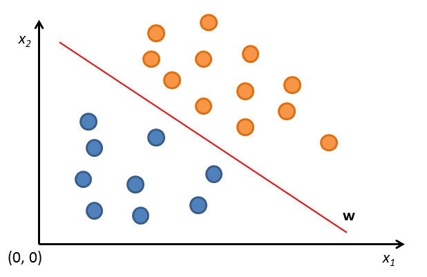
In the above image a set of supervisions is represented in a two dimensional features space, a.k.a. \(\mathbb{R}^2\). Each vector \(\mathbf{x}_i\) is colored either blue or orange. The colors represent the classes.
As you can see, using this features space, supervisions are naturally distributed in two different sets inside \(\mathbb{R}^2\). So, a learner in such space is represented by a line \(\mathbf{w}\) that divides the two sets of supervisions, orange-colored and blue-colored. Orange-colored supervisions are above \(\mathbf{w}\); Blue-colored supervisions are below \(\mathbf{w}\).
For this problem, the hypothesis space is the set of all hyperplanes in \(\mathbb{R}\). The learning process tries to discover the hyperplane \(h\) that divides supervisions in their classes.
Conclusions
Summarizing, we just reduced the problem of supervised learning in a simplier problem, which is the selection process of an hyperplane in \(\mathbb{R}^d\). We can identify different types of supervised learning (i.e. Neural Networks, Support Vector Machines, and so on), that differ by the algorithm that is used to find the hyperplane.
As we saw, the selection process of the features space is a core process. If we choose a features space in which the supervisions are not separable, the learning process will becomes harder and an optimal solution could not exist.
In the next part of this series of posts, we are going to explore some other interesting features of machine learning, i.e. training, validation and testing processes, generalization, overfitting and many others.
Stay tuned.